Learn SQL Application
Intro
SQL as declarative lanuguage is used to tell the machine what we want to get and machine needs to figure out the computation tasks to provide quieried result. In this post I put my notes and examples that helps me to understand different aspects of SQL. There is also the application for learning SQL demonstrated in the Demo section and its source code linked below.
In this section I describe following concepts:
- Database Schema
- Primary and foreign key
- Query types
- Constraints
- Stored procedures
- Temporary table
- Normalization
- One-to-many
- Many-to-many
- Variables
- OLTP and OLAP
- Functions
- Transaction
- Privileges
- Char vs varchar vs nvarchar
- Unique records without DISTINCT
- Common Table Expression
- SQL Delta
- Running Total
- Window alias
- Dates
- Cursors
- SQL performance
Also some SQL syntax elements:
- SELECT INTO
- LIKE
- INDEX
- VIEW
- DISTINCT
- COUNT
- JOIN
- SELF JOIN
- USING
- UNION
- EXCEPT
- INTERSECT
- ORDER BY
- LIMIT
- TOP
- WHERE
- CASE
- GROUP BY
- HAVING
- IN
- OVER
- OFFSET
- FETCH
- EXISTS
- IS NULL
- IS NOT NULL
- IFNULL
- CAST
- CONCAT
- UNPIVOT
- TRUNCATE TABLE
- UPDATE
- ANY
Terminology and general aspects
- Database Schema:
- the strucutre around the data and corresponding data relationships,
- we can have two different approaches on data schema:
- a method of how schema gets defined impacts the further behaviour:SCHEMA ON READ SCHEMA ON WRITE In an unstructured data store we apply a schema only when the data gets read. Forces a structure as a condition before data gets written Data lives in unordered state - and we apply the structure to the query code.
- DB schema has a big impact on quering time.OLTP OLAP When a series of table connected with PKs then db is designed for reading and mostly for writing single record at a time. if there is a central table connected to keys of surrounding tbales then it's designed to keep read output highly efficient. For transactional databs like Salesforce or any ERP. For high scale information delivery.
- Table schema is a different concept on the way of building the fileds and establishing data types for each one. - Primary key - a column or columns combination that idetifies a specific row uniquely. It implies NOT NULL constraint and hast to be UNIQUE. In case of multiple columns as piramry key, we deal with so-called composite key that can encasulate even up to 32 columns.
- Foreign key - a column that contains a primary key from another table's field. This way, we build the relationship between tables.
- In above example pk stands for primary key and fk stands for foreign key.customers
- customer_id: pk integer
- phone: string
- email: stringorders
- order_id: integer
- status: string
- customer_id: fk integer
- In one to many relationship: one customer can have many orders, so we can find one customer multiple times in the orders table.
- As per one to many relationship, one order cannot have multiple customers.
orders tableorder_id status customer_id 1 completed 1 2 completed 1 3 cancelled 3 4 pending 1 - Db engine executes query in the sequence as below:
1. FROM, JOIN - it determines data table(s).
2. WHERE - records filtering.
3. GROUP BY - records grouping.
4. HAVING - groups filtering.
5. SELECT - columns filtering.
6. ORDER BY - results sorting.
- There are different types of SQL queries:
1. DQL - Data Query Language:
-SELECT.
2. DML – Data Manipulation Language:
-INSERT,UPDATE,DELETE.
3. DDL – Data Definition Language:
-CREATE,ALTER,DROP,RENAME,TRUNCATE.
4. DCL – Data Control Language:
-GRANT,REVOKE.
5. TCL - Transaction Control Language:
-COMMIT,ROLLBACK,SAVEPOINT.
- Constraints - we put them as the limits on the data types of the table. It can be specified while creating or altering the table statement.
Here they are:
- NOT NULL - prevents from keeping nulls in the column.
- CHECK - limits the value range that can placed in the column for instance:
Age INTEGER, CHECK (AGE>=18).
- DEFAULT - provides default value to all records unless other value specified.
- UNIQUE - prevents from storing duplicates within a column.
- PRIMARY KEY - sets pk on a column.
- FOREIGN KEY - sets fk indicating pk of a table in the relationship.
- Data integrity - defines the accuracy as well as the consistency of the data stored in a database. Once data integrity ensured then any addition or deletion of data from the table will not create any mismatch in the relationship of the tables.
- Stored procedure - saved SQL code so that it can be reused anytime with or without parameters:
- stored procedure syntax:CREATE PROCEDURE procedure_name AS sql_statement GO;
- executing stored procedure:EXEC procedure_name
- here how it looks like with parameters:CREATE PROCEDURE SelectAllEmployees @City nvarchar(30), @PostalCode nvarchar(10) AS SELECT * FROM employees WHERE City = @City AND PostalCode = @PostalCode GO;
- calling it with parameters:EXEC SelectAllCustomers @City = 'Cracow', @PostalCode = '30-708';
- They can be used as a modular programming which means creating once, storing and calling many times whenever required.
- This supports faster overall query performance.
- There is also such thing as recursive stored procedure which calls itself until it reaches some boundary condition. It allows to reuse the same code any number of times. - Stored procedure vs function:
Stored procedure Function Pre-compiled objects which are compiled for the first time and its compiled format is saved. Gets compiled and executed every time whenever it is called. Returning a value is optional. The function must return a value. Can have input or output parameters. Can have only input parameters. Procedures cannot be called from a Function. Functions can be called from Procedure. Allows SELECT as well as DML(INSERT/UPDATE/DELETE) statements. Function allows only SELECT statement in it. Procedures cannot be utilized in a SELECT statement. Function can be embedded in a SELECT statement. Stored Procedures cannot be used in the WHERE/HAVING/SELECT line. Functions can be used in the WHERE/HAVING/SELECT line. An exception can be handled by try-catch block. Try-catch block cannot be used in a Function. We can use Transactions in Procedure. We can't use Transactions in Function. Functions return tables that can be treated as another rowset. This can be used in JOINs with other tables. Functions cannot modify the data received as parameters.
Char vs varchar vs nvarchar
- char:
- string storage with fixed size,
- the max number of characters is 255,
- because of fixed size, it uses static memoru allocation,
- much faster than varchar. - varchar:
- string storage with variable size,
- the max number of character can reach up to 65535 characters,
- because of variable size, it uses dynamic memory allocation,
- much slower than char. - nvarchar:
- while varchar stores data in non-Unicode encoding, nvarchar stores data in a Unicode encoding.
Normalization
- Normalization is the db designing process where we aim for minimizing any data redundancy. Redundancy of data means there are multiple copies of the same information spread over multiple locations in the same database.
- There are 3 forms of the normalizaton where each consecutive normal form depends on the previous one:
✓ First normal form (1 NF),
✓ Second normal form (2 NF),
✓ Third normal form (3 NF),
where db is considered the third normal form if it meets the requirements of the first 3 normal forms. - In 1 NF wa aim to keep only atomic information. Here is the example which violates the 1NF as it contains more than one value for the department column:
Assignment table
- Definitely we should be avoiding breaking down department column into a set of new columns like department1, department2, department3. This is what we call repeating groups and it's one of the biggest design error.assign_id emp_name emp_age department 1 Artur 20 IT, DevOps 2 John 40 IT, DevOps, DataLab
- In order to reach 1 NF, we need to split the table into two tables so that each record can be unique and each cell contains an atomic, undividable value:
Departments table and assignment table
- We can move on and make the table in 2 NF and 3 NF.dep_id dep_name 1 IT 2 DevOps 3 DataLab assign_id emp_name emp_age dep_id 1 Artur 20 1 2 Artur 20 2 3 John 40 1 4 John 40 2 5 John 40 3
- In 2 NF, we care about having single column primary key. In our example, the assignment table has a single-column primary key i.e. assign_id.
- In 3 NF, we get rid of any dependencies where non-key columns may depend on non-key columns. Dependecy can exist only on primary key column. In order to achieve it, we need to take the non-key column emp_age which depends on the non-key column emp_name into separate table named employees.
Employees table and assignment table
- With that solution what we get is many-to-many relationship where many employees can be assigned to one or more departments.emp_id emp_name emp_age 1 Artur 20 2 John 40 assign_id emp_id dep_id 1 1 1 2 1 2 3 2 1 4 2 2 5 2 3
- Assignment table plays then a role of the connector table that manages many-to-many relationship.
- Assignment table has following columns:
✓ assign_id which is the primary key (unique),
✓ emp_id which is the foreign key (non-unique),
✓ dep_id which is the foreign key (non-unique).
- When we care about keeping table normalized we get a set of benefits:
- better db organization,
- more tables with smaller rows,
- easy modification,
- reduction of redundant and duplicate data.
- ensuring data integrity.
One-to-many relationship
- When one record from table A can have multiple corresponding records in table B.
- Lets take Products and Categories tables:
 source: sqlpedia.pl
- one category can be assigned to many products, however one product cannot be assigned to many categories.
Many-to-many relationship
- This kind of relationship can be handled by connector table that breaks relationship into two relationships of one-to-many. As the example, let's take order system, where each product can be ordered many times in different orders.
- Here are Orders and Products tables connecter with one-to-many relationships with Order Details table.
 source: sqlpedia.pl
Variables
- We can set variable data type, assign a value to it, and use it in the code:
DECLARE @TestVariable AS VARCHAR(100)
SET @TestVariable = 'This is an example string.'
PRINT @TestVariable
- We can display variable value with SELECT or PRINT statements.
- We can also use SELECT statement in order to assing a value to a variable:
DECLARE @CarName AS NVARCHAR(50)
SELECT @CarName = car_model
FROM db.cars
WHERE car_id = 1492
PRINT @CarName
- or:DECLARE @NumCars AS INT SET @NumCars = (SELECT COUNT(*) FROM db.cars)
- When we assign multiple-rows SELECT result to a variable, the assigned value to the variable will be the last row of the result set.
- It's important to remember that local variable scope expires at the end of the batch which can be determined by GO statement.
- Thus the lifecycle of variable
@TestVariabledetermines with GO statement line. In other words, the variable which is declared above the GO statement line can not be accessed under the GO statement. - Variable scopes:
Local Variable Global Variable A user declares the local variable. The system maintains the global variable. A user cannot declare them. By default, a local variable starts with @. The global variable starts with @@. Can be used or exists inside the function. Can be used or exists throughout the program.
OLTP and OLAP
| Online Transaction Processing (OLTP) | Online Analytical Processing (OLAP) |
| Online database modifying system. | Online database data retrieving system. |
| Uses traditional DBMS. | Uses the data warehouse. |
| Insert, Update, and Delete operations. | Mostly select operations. |
| Queries are standardized and simple. | Complex queries involving aggregations. |
| Tables are normalized. | Tables are not normalized. |
| Transactions are the sources of data. | Different OLTP databases become the source of data for OLAP. |
| Maintains data integrity constraint. | Doesn't get frequently modified. Hence, data integrity is not an issue |
| Designed for real time business operations. | Designed for analysis of business measures. |
Functions
- SQL has many built-in functions that can be categorised in two categories:
Scalar function Aggregate function Window function Returns a single value from the given input value. Performs calculations on a group of values and then return a single value. Computes values over a group of rows and returns a single result for each row. input: 1 record
output: 1 recordinput: n records
output: 1 recordinput: n records
output: n recordsLCASE()
UCASE()
LEN()
MID() / SUBSTRING()
LOCATE() / CHARINDEX()
ROUND()
NOW()
FORMAT()
INSTR()
CONCAT()
REPLACE()
YEAR()SUM()
COUNT()
AVG()
MIN()
MAX()
FIRST()
LAST()... - Windows:
- Executes a specific function based on the moving window that encapsulates one or N records at a time,
- Includes an OVER clause, which defines a moving window of rows around the row being evaluated.
SELECT
  [Month]
  ,[SalesTerritoryKey]
  ,[SalesAmount]
  ,[WindowFunction] = SUM([SalesAmount])
			    OVER (PARTITION BY [SalesTerritoryKey]
			      	ORDER BY [Month]
			      	ROWS BETWEEN 1 PRECEDING AND CURRENT ROW
			  	)
FROM    [CTE_source]
ORDER BY [SalesTerritoryKey],[Month];
mssqltips.com
- For computing moving averages, rank items, cumulative sums.
- Can be put in SELECT or ORDER BY lines.
- There are 3 main terms when working with analytic functions: partition, window and current record:
 mssqltips.com
Window functions:
- They allow to refer to a value of an indicated record different than the current one.
- LAG:
- returns a value of a specific field from the preceiding record of a current partition,
- when LAG function called for the first record of a current partition, it returns NULL,
- example:SELECT CAST(DueDate AS DATE) AS DueDate, OrderID, Total, LAG(Total) OVER (PARTITION BY DueDate ORDER BY DueDate) AS PreviousDueDateTotal FROM tblSales ORDER BY DueDate
- year to year comparison:WITH cte_company_orders AS( SELECT year, curr_year, LAG(current_year, 1) OVER (ORDER BY year) AS prev_year FROM company_details) SELECT year, curr_year, prev_year, ROUND( (curr_year - prev_year) / (CAST(prev_year AS NUMERIC)) * 100 ) AS perct_diff FROM cte_company_orders- With LAG we take a value from previous records for each following record.
- It surves for calculating year to year growth calculation where we can get value for a current record an the preceding one.DueDate OrderId Total PreviousDueDateTotal 2008-06-14 71776 87.08 NULL 2008-06-14 71832 3953160.1 87.08 2008-06-14 71833 22 3953160.1 2008-06-17 71835 9102.11 NULL 2008-06-17 71835 5512.94 9102.11 - LEAD:
- returns a value of a specific field from the following record of a current partition,
- when LEAD function called for the last record of a current partition, it returns NULL. - FIRST_VALUE:
- returns the first value of a speciic field of a current partition,
- LAST_VALUE:
- returns the last value of a specific field of a current partition.
Rank functions:
- ROW_NUMBER()
SELECT *
FROM (
  SELECT
    *,
    ROW_NUMBER() OVER (PARTITION BY dept_name ORDER BY emp_salary) r_numb
  FROM employees) e
WHERE e.r_numb < 2
- query shows first two employees with the smalles salary per department.emp_id emp_name emp_salary dept_name r_numb 5 Krzysztof 7,100.00 Admin 1 3 Johnny 9,600.00 Admin 2 4 Rick 5,500.00 HR 1 1 Artur 7,500.00 IT 1 6 Caroline 15,500.00 IT 2 ... ... ... ... ... - DENSE_RANK()
SELECT customer_id, events
FROM (
	SELECT customer_id,
	  COUNT(*) AS events,
	  DENSE_RANK() OVER (ORDER BY COUNT(*)) AS rank
	FROM fact_events
	WHERE client_id = 'mobile'
	GROUP BY customer_id) subquery
WHERE rank <= 2
ORDER BY 2 ASC
- Above query finds bottom 2 companies with dense rank.
- DENSE_RANK() keeps counting in the consecutive sequence even though there might be some ties along the way.
- The order of the ranking is ascending by defualt.
- Sub-query outcome:
- and we take the first 3 records from the sub-query to fulfile WEHERE rank <=2customer_id events rank a 4 1 b 4 1 c 7 2 d 14 3 e 21 4 - RANK and DENS_RANK:

source: techTFQ
- RANK() alone skpis every duplicated records.
Analytic function:
- NTILE(x), where x is number of equal ranges in which we want to classify the records:
SELECT
	category_name,
	month,
	FORMAT(net_sales,'C','en-US') net_sales,
	NTILE(4) OVER(
		PARTITION BY category_name
		ORDER BY net_sales DESC
	) net_sales_group
FROM
	sales.vw_netsales_2017;
- outcome:

source: techTFQ
- that way we got 4 evenly distributed buckets. - Getting the category with lowest value using ntile:
SELECT shop_id, total_order
FROM (
  SELECT
    shop_id,
    SUM(total) AS total_order,
    NTILE(50) OVER (ORDER BY SUM(total)) AS ntile
  FROM shops
  WHERE customer_placed_order BETWEEN '2020-05-01' AND '2020-05-31'
  GROUP BY shop_id
)
WHERE ntile=1
ORDERBY 2 DESC
- With ORDER BY in OVER() we make sure SUM(TOTAL) is ordered ascendingly.
- Entire ordered SUM(TOTAL) column will be divided into 50 evenly distributed buckets.
- Taking first bucket ensures us we take into an account only lowest generating shops.
- NTILE takes 50 as we want to get all shops <= 2% of shop's revenue.
- If I had to take 1% of shop's revenue then I would go with NTILE(100).
Transaction
- Single set of task performed on a database in logical manner.
- It inlcudes operations like creating, updating, deleting.
- There are 4 transaction controls:
- commit: saving all changes made by a transaction,
- rollback: reverts all changes made by a transaction and the database remains as before,
- set transaction: setting a transaction's name,
- savepoint: sets the point where a transaction can roll back to.
Privileges
- A db admin can GRANT or REVOKE privileges to or from users of database.
- GRANT command provides database access to a user:
GRANT SELECT
ON employee
TO user1
- This command grants a SELECT permission on employee table to user1.
- REVOKE removes database access from a user:
REVOKE SELECT
ON employee
FROM user1
- This command will REVOKE a SELECT privilege on employee table from user1.
- user1 will lost privilege on employee table only when everyone who granted the permission revokes it.
SELECT INTO
- Statement that copies data from a table to the new one.
SELECT *
INTO newtable [IN externaldb]
FROM oldtable
WHERE condition;
- Here is how to use INSERT INTO SELECT:
INSERT INTO Customers (CustomerName, City, Country)
SELECT SupplierName, City, Country FROM Suppliers;
WHERE Country='Poland';
| SELECT INTO | INSERT INTO SELECT |
| Used when the table doesn't exist. | Used when the table exists. |
| For single task like creating temporary table, ad hoc reporting or backup table. | Used regularly to appending rows to tables. |
| Copies all data with data types to the newly-created table. | Data types in source and target tables must match. |
Temporary table:
- Exists temporarily storing a subset of data from a normal table.
- You filter data once and store the result in a temporary table instead of filtering the data again and again to fetch the subset.
- Temporary table needs to be named with '#' prefix.
- We can make use of SELECT INTO to create a temporaty table:
SELECT name, age, gender
INTO #FemaleStudents
FROM student
WHERE gender = 'Female'
- We can keep it inside a stored procedure:
CREATE TABLE #MaleStudents(
  name VARCHAR(50),
  age INT,
  gender VARCHAR (50)
)

CREATE PROCEDURE spInsertStudent (@Name VARCHAR(50), @Age INT,  @Gender VARCHAR(50))
AS
BEGIN
  INSERT INTO #MaleStudents VALUES (@Name, @Age, @Gender)
END

CREATE PROCEDURE spListStudent
AS
BEGIN
  SELECT * FROM #MaleStudents
  ORDER BY name ASC
END

EXECUTE spInsertStudent Bradley, 45, Male
EXECUTE spListStudent
source: codingsight.com
- The 1st procedure inserts a new student record with the name: Bradley, age:45, gender: Male.
- The 2nd procedure selects all the records from the table in the ascending order of name. - When a temporary table created, it gets an unique identifier in order to differentiate between the temporary tables created by different connections. You can perform operations on the temporary table via the same connection that created it.
- A temporary table is automatically deleted when the connection that created the table is closed.
LIKE
- LIKE operator is used for pattern matching.
- It can be used with wildcards:
- "%"" - matches zero or more characters.
SELECT *
FROM employees
WHERE emp_surname LIKE 'S%'
- "_" - matches exactly one character.
VIEW
- It's a virtual table based on the result of any SQL statement.
- A view contains all you need in every other table: rows and columns and fields can come from one or more real tables.
- While creating views, we can apply
WHEREorJOINstatements to keep the data as if it comes from one single table. - Here is the syntax for view creating:
CREATE VIEW view_name AS
SELECT column1, column2, ...
FROM table_name
WHERE condition;
- end here is how to query a view:SELECT * FROM view_name - With views we can restric users from being able to check some confidential data.
In a view we just define what columns are visible. The columns we want to keep invisible, we don't include them into the view while creating.
For example, lets say we have the employees table data schema:
- id: numeric
- first_name: string
- last_name: string
- salary: numeric
Let's assume that column salary is confidential and has to be restricted from viewing:CREATE VIEW emloyess_details AS SELECT first_name, last_name, FROM employess WHERE last_name LIKE 'S%';- When we wat to check salary somehow:SELECT last_name, salary FROM emloyess_details WHERE last_name LIKE 'S%';- Querying the viewemloyess_detailsforsalaryfield raises an error. - It aslo simplifies queries hiding their complexity made with UNION, JOIN etc.
- Let's have a look at differences between a view and the actual table:
- The difference between a view and a table is that views are definitions built on top of other tables (or views), and do not hold data themselves.
- A view hides the complexity of the database tables from end users. Essentially we can think of views as a layer of abstraction on top of the database tables.
- If data is changing in the underlying table, the same change is reflected in the view.
- Views takes very little space to store, since they do not store actual data.
- Views can include only certain columns in the table so that only the non-sensitive columns are included and exposed to the end user. - We can modify the data with using views but under following conditions:
- there is no groupping with GROUP BY in the view,
- there is no DISTINCT in view's definition,
- there are no expressions in view's definiton,
- only one base table is being updatred through a view,
- modified values are in line with base table field constraints.
In all views that can modify the data we should implement WTH CHECK OPTION clause so that we can prevent users from overriding any changes he has just performed.
INDEX
- An index is used to speed up searching in the database by reducing records amount to be scanned.
- An index helps to speed up
SELECTqueries andWHEREclauses, but it slows down data input, with theUPDATEand theINSERTstatements. - In order to set an index we use
CREATE INDEXstatement, which allows us to name the index as well as to specify a table and a column that we want to get indexed:CREATE INDEX index_name ON table_name (column_name);
- Updating a table with indexes takes more time than updating a table without (because the indexes also need an update). So, only create indexes on columns that will be frequently searched against.
- When not to use indexes:
- on small tables,
- on tables that have frequent, large updates or insert operations,
- on columns that contain a large number of NULLs,
- on columns that are frequently manipulated.
- Here is how to use it:
- creating index:CREATE INDEX employees_last_name_idx ON employees (last_name);- using indexed column in the select query:SELECT * FROM employees WHERE salary > 10000 AND last_name = "Smith"- We uselast_nameindexed column within the WHERE caluse along withsalarywhich speeds up performing the query.
- It simply works like an index in the book where the index key (indexed column name) points to every respective record keeping value from the rest of non-key columns. What is very important, index keys are sorted.
- If the table is not indexed then database server needs to go through all records to execute any query.
- It's recommended to use at leat one indexed column when groupping wiht GROUP BY. - The most optimal number of indexes put on the same table is not greater than 10. - We can also index multiple columns, however it takes very long to set it up for the db engine.
- We can say that there are two types of indexes:
- It is important to mention here that inside the table the data will be sorted by a clustered index.Clustered Index Non-Clustered Index Defines the order of storing data in the table Doesn't define the order of data inside the table As data always can be stored in one way, there can be only one clustered index. When creating a table, the primary key constraint automatically creates index on that column. In fact, non-clustered index is stored at different place than table data is stored. This allows for more than one non-clustered index per table. Clustered indexes only sort tables. Therefore, they do not consume extra storage. Non-clustered indexes are stored in a separate place from the actual table claiming more storage space. Fast performance. Slower performance as it requires additional lookup between index sotrage and acutal table.
- However, inside the non-clustered index data is stored in the specified order.
- The non-clustered index contains column values on which the index is created and the address of the corresponding records in the actual table. - Here is how it works:
- When a query is run against indexed column, the database will first go to the index and look for the address of the corresponding row in the table. It will then go to that row address in the table and fetch other column values.
DISTINCT
- Using when we wan to get unique values from a given column.
SELECT DISTINCT name
FROM students
- Aggregating function COUNT() counts duplicates. To count only unique values we need to put DISTINCT prior to COUNT() argument:
SELECT COUNT(DISTINCT client_region)
FROM tblSales
- all aggreagating functions ignore NULL values by default,
- however, with syntax: COUNT(*) we calculate both duplicates and nulls,
- all aggreagating functions take all values including deuplicated ones - we can prevent this using DISTINCT keyword,
- even though all aggregating functions can accept unique values, keyword DISTINCT is most often used with COUNT(). - Using COUNT(DISTINCT col_name) to get first/second... max value:
SELECT name, price
FROM sales AS A
WHERE 0 = (
    SELECT COUNT(DISTINCT price)
    FROM sales AS B
    WHERE B.price > A.price
)
- The sub-query in the WHERE clause is being performed for each and every record from the outer query.
- For every record from the outer query, there is a check in WHERE clause: if 0 equals sub-query outcome then put outer query recod into the result set one at a time.
- When we want to get products with second biggest price we would need to replace 0 with 1 in the WHERE clause etc.
JOIN
- Join is the keyword needed when quering more than one table.
- While joining, we need to define on what columns (of both tables) we will be keeping tables joined.
- Usually, we use primary key of one table matching it with its corresponding foreign key in another table.
- There are a few kind of joins:
- (INNER) JOIN: returns rows when there is a match in rows between the tables.
- LEFT (OUTER) JOIN: returns all the rows from the left table regardless if there is a match or a null from the right table.
- RIGHT (OUTER) JOIN: returns all the rows from the right table regardless if there is a match or a null from the left table.
- FULL (OUTER) JOIN: returns all the rows from the left-hand side table and all the rows from the right-hand side table.
- CROSS JOIN: joins every row of one table with every row of another table. A very complex operation when cross joining more than 2 tables. Requiring from the performance perspective. - Let's take two table schemas for an example:
tblVideo
- video_id: PRIMARY KEY integer
- author_id: integer
- video_duration: floattblView
- video_id: FOREIGN KEY integer
- viewer_id: integer
- viewer_timewatch: float - Inner join example:
How many publishers have at least one viewer?SELECT COUNT(DISTINCT vd.author_id) FROM tblVideo vd INNER JOIN tblView vw ON vd.video_id = vw.video_id
- It doesn't count authors whose videos are not in the tblView.
- If I want to count disctinct author's id, I wouldn't need any JOINs and do select only on tblVideo. - Left join example:
- Here is the snippet of data schema:
 source: toptal.com
SELECT i.Id, i.BillingDate, c.Name, r.Name AS ReferredByName
FROM Invoices i
 LEFT JOIN Customers c ON i.CustomerId = c.Id
 LEFT JOIN Customers r ON c.ReferredBy = r.Id
ORDER BY i.BillingDate ASC;
- With LEFT JOIN we make sure that all the invoices will be returned no matter what (in case of any NULLs within Customers table).
- First LEFT JOIN joins customer id pk with customer id fk in the Invoices table.
- Second LEFT JOIN joins customer id pk with cusotmer id fk in the Customer table.
- ORDER BY orders outcome by date. We can append ASC/DESC if ascending or descending ordering. - We can join multiple tables:
SELECT column1, column2
FROM TableA
JOIN TableB ON TableA.Column3 = TableB.Column3
JOIN TableC ON TableA.Column4 = TableC.Column4
- We can also join a table with itself what we call self join
SELECT DISTINCT E.FullName
FROM EmployeeDetails E
INNER JOIN EmployeeDetails M
ON E.EmpID = M.ManagerID;
- We are using different aliases to differentiate tables on join.
- This way we fetch those emps whose id are present in the ManagerID column. - Selecting the columns on which join is applied:
SELECT t1.main_col AS col_A, t2.main_col AS col_B
FROM tab1 t1
FULL OUTER JOIN tab2 t2
ON t1.main_col = t2.main_col
- we just need to alias the columns properly to fetch them boht separately.
- result:
col_A col_B Null 1231235 Null 5234214 4434431 4434431 2221222 2221222 9765675 Null 7654565 Null - Cross join using 1 = 1 as join condition:
- It's simply doing a cross join, which selects all rows from the first table and all rows from the second table and shows as cartesian product, i.e. with all possibilities.
- Putting in 1=1 is like saying "1=1 is always true, do don't eliminate anything". - Greater/Lower than in the ON condition:
- having below table:
and joining table to itselfname price a 10 b 15 c 20 d 20 SELECT * FROM products AS A JOIN products AS B ON A.price > B.price
we get
- query with a such condition in JOIN ON, for every record of A table assigns all of the records of B table where price is lower.name price name price b 15 a 10 c 20 a 10 c 20 b 15 d 20 a 10 d 20 b 15 - Multiple conditions in ON caluse:
SELECT u1.*
FROM users u1
JOIN users u2
ON u1.user_id_sender = u2.user_id_sender
AND u1.user_id_receiver = u2.user_id_receiver
- we self join the same table of users,
- we use combination of two columns as a combined key.
USING
- USING clause comes in use while working with JOIN and can be used instead of ON clause.
- When we use USING clause, that particular column name should be present in both tables, and the SELECT query will automatically join those tables using the given column name in USING clause.
- Here comes the example:
SELECT e.emp_id, e.last_name, d.loc_id
FROM emploees e
JOIN departments d
USING(dep_id);
- in tables employees and departments, dep_id column is the mutual one. - Another example with delete query:
DELETE FROM tab1
USING tab2
WHERE tab1.k = tab2.k
UNION
- Merges the contents of two structurally-compatible tables into a single combined table removing duplicated records.
- There is also UNION ALL that does the same things but keeps duplicated records.
- Performance of UNION ALL is better than UNION, since UNION requires the server to do the additional work of removing any duplicate.
- Here is how to use it:
SELECT employee_id, first_name, last_name, 'Employee' AS status
FROM employees
UNION
SELECT visitor_id, first_name, last_name, 'Visitor' AS status
FROM visitors
- note that colums selected from both tables have to be in sync with each other. - We can use multiple UNION statements in a one query.
EXCEPT
- Allows to fetch values from one table that are not in another table.
CREATE TABLE test_a(id INTEGER);
INSERT INTO test_a(id) VALUES (10);
INSERT INTO test_a(id) VALUES (20);
INSERT INTO test_a(id) VALUES (30);
INSERT INTO test_a(id) VALUES (40);
INSERT INTO test_a(id) VALUES (50);

CREATE TABLE test_b(id INTEGER);
INSERT INTO test_b(id) VALUES (10);
INSERT INTO test_b(id) VALUES (30);
INSERT INTO test_b(id) VALUES (50);

SELECT * FROM test_a
EXCEPT
SELECT * FROM test_b;

----------------------
20, 40
- 20 and 40 are the values that are not present in test_b table.
INTERSECT
- Fetchs common records between two tables:
SELECT * FROM EmployeeSalary
INTERSECT
SELECT * FROM ManagerSalary;
LIMIT
- Limiting select query results to specific numbers of records:
SELECT *
FROM (
	SELECT *
	FROM employees
	ORDER BY salary DESC )
LIMIT 10;
- We fetch 10 highest salaries in employees tabel.
- We use subquery meaning we emebd one select into another.
TOP
- We can select x top records:
- let's assume we have customers table and the fields customer_id,
- let's fetch first 100 odd cutomer_id values,
- there, we use WHERE clause to filter fetched rows, this clause allows AND as well as OR operators,SELECT TOP 100 customer_id FROM customers WHERE customer_id % 2 = 1 ORDER BY user_id
- Clause WHERE can also have BETWEEM operator:SELECT * FROM employees WHERE date_of_joining BETWEEN '2020/01/01' AND '2020/12/31';
- BETWEEN in WHERE clause is inclusive.
- When it comes to dates, we can extract what we want:SELECT * FROM employees WHERE YEAR(date_of_joining) = '2020'
GROUP BY
- Groups rows into categories within a column we indicate:
SELECT COUNT(CustomerID), Country
FROM Customers
GROUP BY Country
HAVING COUNT(CustomerID) > 3;
and then we can run any aggregating function for a particular category.
- We count all customers for a specific country but we display countires where count is bigger than 3.
- We use GROUP BY when some aggregating function in select line like COUNT, SUM, AVERAGE.
- When using GROUP BY, in the select line we can use only aggregating functions and columns that are enclosed by GROUP BY.
- We can create some sub-groups for example:GROUP BY Country, Region
- HAVING simply puts filter on COUNT(CustomerID) outcome column.COUNT(CustomerID) Country 9 Brazil 11 France 11 Germany 5 Mexico 5 Spain 7 UK 13 USA 4 Venezuela
- WHERE vs HAVING:
- When GROUP BY is not used, then WHERE and HAVING clauses works the same.
- When GROUP BY is used, then WHERE clause is used to filter records from a result and filtering works before any grouping. HAVING clause is used to filter values from a group. - We can even have some calculations within HAVE:
WITH cte_pays AS(
	SELECT
	    date,
	    SUM(CASE WHEN a.paying_customer = 'yes' THEN d.downloads END) AS paying_sum,
	    SUM(CASE WHEN a.paying_customer = 'no' THEN d.downloads END) AS non_paying_sum
	FROM user_dimension u
	LEFT JOIN acc_dimension a ON u.acc_id = a.acc_id
	LEFT JOIN download_facts d ON u.user_id = d.user_id
	GROUP BY d.date
	ORDER BY d.date ASC)
SELECT *
FROM cte_pays p
GROUP BY
	p.date,
	p.paying_sum
	p.non_paying_sum
HAVING (p.non_paying_sum - p.paying_sum) > 0
ORDER BY p.date ASC
- with CASE WHEN and SUM() we calculate another columns based on the old column: downloads,
- the first one sums all values when condition paying_customer = 'yes',
- the another one sums all values when condition paying_customer = 'no'.
Referencing to the same table more than once:
- Here is the employees table:
Emp_Id Emp_name Salary Manager_Id 10 Anil 50000 18 11 Vikas 75000 16 12 Nisha 40000 18 13 Nidhi 60000 17 14 Priya 80000 18 15 Mohit 45000 18 16 Rajesh 90000 Null 17 Raman 55000 16 18 Santosh 65000 17 - Lets fetch all rows with WHERE clause on a.manager_id = b.emp_id:
SELECT *
FROM Employee a, Employee b
WHERE a.manager_id = b.emp_id
- Note there is no Rajesh in the outcome as he has no manager above him. Rajesh appears only as the manager for other employees.10 Anil 50000 18 18 Santosh 65000 17 11 Vikas 75000 16 16 Rajesh 90000 Null 12 Nisha 40000 18 18 Santosh 65000 17 13 Nidhi 60000 17 17 Raman 55000 16 14 Priya 80000 18 18 Santosh 65000 17 15 Mohit 45000 18 18 Santosh 65000 17 17 Raman 55000 16 16 Rajesh 90000 Null 18 Santosh 65000 17 17 Raman 55000 16 - Let's group managers counting average salary:
SELECT b.emp_id AS "Manager_Id", b.emp_name AS "Manager", AVG(b.salary) AS "Avg_Salary_Under_Manager"
FROM employees a, employees b
WHERE a.manager_id = b.emp_id
GROUP BY b.emp_id
ORDER BY b.emp_id;
Manager_Id Manager Average_Salary_Under_Manager 16 Rajesh 65000 17 Raman 62500 18 Santosh 53750
CASE
- We can use Case to give some conditons:
- assuming we have students table and lastname filed and we want to update some records:
UPDATE dbo.students
SET lastname =  CASE
	 WHEN lastname = 'aaa' THEN 'bbb'
	 WHEN lastname = 'ccc' THEN 'ddd'
	 WHEN lastname = 'eee' THEN 'fff'
	 ELSE lastname
	END
WHERE lastname IN ('aaa', 'ccc', 'eee')
- it's very important to enclose WHERE clause in the queries,
- if we omit the WHERE clause, all records will get updated. - Embeding CASE WHEN in SUM():
- using orders table we have fields like ship_country and status,
- we want to show the number of shipped orders by country,
- the order is shipped if the status is “shipped” or “delivered:
SELECT ship_country,
    SUM(CASE
      WHEN status = 'shipped' OR status = 'delivered' THEN 1
      ELSE 0
      END) AS order_shipped
FROM orders
GROUP BY ship_country;
- the code assigns 1 to all records where the status is either "shipped" or "delivered",
- rest of the records with different status get 0 assigned.
- another example to count percentage:
SELECT SUM(CASE WHEN CAST(order_cost AS INT) > 500 THEN 1 ELSE 0 END) * 100.0 / COUNT(*) AS percentage_orders_over_500 FROM orders - Embeding CASE WHEN in COUNT():
SELECT
    	COUNT(CASE WHEN status = "open" THEN user_id ELSE NULL END) / CAST(COUNT(*), FLOAT) AS ratio
FROM users
WHERE country = "USA"
- if the status is equal to 'open' then there is user_id value in COUNT() input.
- If the status is different than 'open' then there is NULL in CCOUNT() input. Function COUNT() ignores NULLs - ratio numerator..
- However function: COUNT(*) count both values and nulls getting all records number - ratio denominator.
- Integer being devided by integer gives 0 - we need to cast at least denominator or numerator into float format in order to get a ratio between 0 and 1.
IN
- The IN operator allows to specify multiple values in a WHERE clause.
- If taken value 'Apple' is in one of given columns then we take rows into results.
| Id | Col1 | Col2 | Col3 |
| 1 | Apple | Null | Orange |
| 2 | Orange | Apple | Strawberry |
| 3 | Strawberry | Apple | Orange |
SELECT *
FROM table
WHERE Col1 IN ("Apple", "Strawberry")
- as the result, we receive 2 records: first and third one.
SELECT *
FROM table
WHERE Col1 NOT IN ("Apple", "Strawberry")
- then we get the second record only.
OVER
- A window function is an SQL function where the input values are taken from a "window" of one or more rows into the results set of a SELECT statement. Window functions are distinguished from other SQL functions by the presence of an OVER clause.
- OVER clause has been added to SQL Server and can be used to determine which rows from the query are applied to the function.
- PARTITION BY clause is used to divide the result set from the query into data subsets, or partitions.
PARTITION BY clause is not used, the entire result set from the query is the partition that will be used.
The window function being used is applied to each partition separately, and the computation that the function performs is restarted for each partition.
Lets have a look at example without OVER and with OVER applied:
SELECT
    emp_id,
    emp_name,
    dept_name,
    emp_salary,
    MAX(emp_salary) OVER () as max_salary
FROM employee
source: sqlservercentral.comemp_id emp_name emp_salary dept_name max_salary 1 Artur 7,500.00 IT 15,500.00 2 Robert 10,000.00 Admin 15,500.00 3 Johnny 9,600.00 Admin 15,500.00 4 Rick 5,500.00 HR 15,500.00 5 Krzysztof 7,100.00 Admin 15,500.00 6 Caroline 15,500.00 IT 15,500.00 ... ... ... ... ...
- This query returns the maximum salary of all records for each record.
- Since a PARTITION BY clause was not used, the entire result set was treated as a single partition.
- Let's apply PARTITION BY clause:SELECT emp_id, emp_name, dept_name, emp_salary, MAX(emp_salary) OVER (PARTITION BY dept_name ORDER BY emp_salary) as max_salary FROM employee
source: sqlservercentral.comemp_id emp_name emp_salary dept_name max_salary 5 Krzysztof 7,100.00 Admin 10,000.00 3 Johnny 9,600.00 Admin 10,000.00 2 Robert 10,000.00 Admin 10,000.00 4 Rick 5,500.00 HR 5,500.00 1 Artur 7,500.00 IT 15,500.00 6 Caroline 15,500.00 IT 15,500.00 ... ... ... ... ...
- Above query has a PARTITION BY clause of the dept_name column, so the max function takes all records assigned to a particular department.
- Additionaly, ORDER BY orders records by emp_salary ascendingly within each partition.
OFFSET
- The OFFSET clause specifies the number of rows to skip before starting to return rows from the query. The FETCH clause specifies the number of rows to return after the OFFSET clause has been processed.
- We must use the OFFSET and FETCH clauses with the ORDER BY clause.
- Skipping the first 10 products and selecting the next 10 products:
SELECT product, price
FROM products
ORDER BY price, product
OFFSET 10 ROWS
FETCH NEXT 10 ROWS ONLY;
EXISTS
- The EXISTS operator is used to test for the existence of any record in a subquery.
- The EXISTS operator returns true if the subquery returns one or more records:
SELECT name
FROM products p1
WHERE EXISTS (
  SELECT 1
  FROM products p2
  WHERE p1.name = p2.name AND p2.price > 15
)
- Above query returns TRUE and lists the suppliers with a product price less than 20.
- In the sub-query we need to have a reference to the table from the outer query.
IS NULL
- Sometimes we want to fetch the nulls, then we use IS NULL in the WHERE clasue:
SELECT c.id AS c_id, pc.id AS pc_id
FROM clients c
FULL OUTER JOIN premium_clients pc
ON c.id = pc.id
WHERE pc.id IS NULL
- checking which elements of the id clomun are sitting in the client table but they are not in the premium_clients table.
- those missing records will be displayed as NULLs in pc_id column. - IS NULL in CASE WHEN:
WITH cte_nulls_to_ints AS(
  SELECT
    *,
    CASE WHEN end_dt IS NULL THEN 1 ELSE 0 END AS int_end_dt
  FROM projects)
SELECT
  SUM(e.salary)
FROM Employees e
JPIN cte_nulls_to_ints c
ON e.id = c.emp_id
GROUP BY e.id
HAVING COUNT(c.project) = SUM(c.int_end_dt)
- we give 1 when there is NULL in the end_dt column.
- HAVIG clasue is a key here as we get only those employees (their ids) only when number of all projects equals the sum of all theis nulls which means they have not finished any project so far. - We can do same exact thing with IS NOT IN and IS NOT NULL:SELECT SUM(salary) FROM Employees e WHERE e.id IS NOT IN( SELECT employee_id FROM projects WHERE end_dt IS NOT NULL )
IS NOT NULL
- In order to ensure not getting Nulls in a queried column we use IS NOT NULL in WHERE clause:
SELECT emp_id, salary
FROM employees
WHERE salary IS NOT NULL
- We can also filter Nulls from multiple columns:
SELECT emp_id, salary, emp_position
FROM employees
WHERE salary IS NOT NULL AND mp_position IS NOT NULL)
IFNULL
- It's a control flow function that accpets two arguments:
SELECT IFNULL(expression_1,expression_2);
- function returns expression_1 if expression_1 is not NULL, otherwise, it returns expression_2.
CAST
- We can use CAST in order to convert data types into other ones.
SELECT CAST(11.25 AS int)
------
11
- in the example above we convert float type into int type.
Unique records without DISTINCT
- We can use GROUP BY in order to eliminate duplicates from a query result:
SELECT surname
FROM employees
GROUP BY surname
- it works because GROUP BY groups all the duplicated values of a specific column into one value (group). - Another option is self joining the table and using NOT EXISTS in the WHERE clause:
SELECT emp_name, emp_address, emp_sex, emp_salary FROM employees e1 WHERE NOT EXISTS (SELECT 1 FROM employees e2 WHERE e2.emp_name = e1.emp_name AND e2.emp_address = e1.emp_address AND e2.emp_sex = e1.emp_sex AND e2.create_date >= e1.create_date)-SELECT 1in the subquery returns constant 1 for every row in the table only when condition in the second WHERE clause is met,
- selecting constant 1 is useful when we want to cheaply determine if record matches condition in the WHERE clause.
Common Table Expression (CTE):
- It's a named temporary result set that exists within the scope of a single statement and that can be referred to later within that statement, possibly multiple times.
- Improves the readability of sql statements.
- When CTE is helpful:
- needing to reference a derived table multiple times in a single query,
- an alternative to creating a view in the database,
- performing the same calculation multiple times over across multiple query components.
- Starts with WITH keyword:
-- define CTE:
WITH Cost_by_Month AS(
SELECT campaign_id AS campaign,
    TO_CHAR(created_date, 'YYYY-MM') AS month,
    SUM(cost) AS monthly_cost
FROM marketing
WHERE created_date BETWEEN NOW() - INTERVAL '3 MONTH' AND NOW()
GROUP BY 1, 2
ORDER BY 1, 2)
SELECT
    campaign, avg(monthly_cost) as "Avg Monthly Cost"
FROM Cost_by_Month
GROUP BY campaign
ORDER BY campaign
source: chartio.com - Using CTEs to handle multiple logic
WITH cte_combined_energy AS (
    SELECT *
    FROM eu_energy
    UNION All
    SELECT *
    FROM usa_energy
    UNION All
    SELECT *
    FROM na_energy),
cte_energy_by_date AS (
    SELECT
        date,
        SUM(consumption) AS total_energy
    FROM cte_combined_energy
    GROUP BY date
    ORDER BY date ASC),
cte_max_energy AS (
    SELECT
        MAX(total_energy) AS max_energy
    FROM cte_energy_by_date)
SELECT
      cebd.date,
      cebd.total_energy
FROM cte_max_energy cme
JOIN cte_energy_by_date cebd
      ON cebd.total_energy = cme.max_energy
- cte_combined_energy: unions all 3 tables (verious length),
- cte_energy_by_date: aggregates values from consumption column and groups the outome by date,
- cte_max_energy: takes max value from aggregation made in the previous cte,
- last select joins cte_energy_by_date and cte_max_energy matching value of max in both.
- This approach is way better than ordering descending and limit the outcome to 1 as we can have more than one record with max_energy value.data total_energy 2021-01-08 6500 2021-01-07 6500
SQL Delta:
- It performs three main functions:
- comparing and optionally synchronizing the structure (schema) of two SQL databases,
- comparing the data in tables (and optionally views) of both the databases,
- displaying the schema of a database. - SQL Delta can generate update scripts to synchronize one database with other database, for both structure and data.
- SQL Delta provides various structure and comparison reports which are saved as HTML. Itpresents an overview of the objects highlighting different, added or deleted.
Running Total
- Here I want to apply running total without any window functions:
- we apply the self inner join:
SELECT t1.ID, t2.ID
FROM demo t1
INNER JOIN demo t2
ON t1.ID >= t2.ID
- there are two join conditions in order to get proper set of data:
1) T1.InvoiceID >= T2.InvoiceID to mix each following invoice id with the rest of prior ones. If there was "=" in the join condition we woul get one by one assigment like: 1 - 1, 2 - 2, 3 - 3 etc...
2) T1.TransactionDate = T2.TransactionDate to include records on the same transaction date.
SELECT   T1.InvoiceID
         ,T2.InvoiceID
         ,T1.TransactionDate
FROM     Sales.CustomerTransactions T1
         INNER JOIN Sales.CustomerTransactions T2
         ON T1.InvoiceID >= T2.InvoiceID
         AND  T1.TransactionDate = T2.TransactionDate
ORDER BY T1.InvoiceID
source: essentialsql.com
InvoiceID InvoiceID TransactionDate 1 1 2021-01-01 2 1 2021-01-01 2 2 2021-01-01 3 1 2021-01-01 3 2 2021-01-01 3 3 2021-01-01 - As we want to calculate the running total we need to get an amount for each invoice and all invoices before:
SELECT   T1.InvoiceID
         ,T1.TransactionDate
         ,T1.TransactionAmount
         ,Sum(T2.TransactionAmount) RunningTotal
FROM     Sales.CustomerTransactions T1
         INNER JOIN Sales.CustomerTransactions T2
         ON T1.InvoiceID >= T2.InvoiceID
         AND  T1.TransactionDate = T2.TransactionDate
GROUP BY T1.InvoiceID
         ,T1.TransactionDate
         ,T1.TransactionAmount
ORDER BY T1.InvoiceID
         ,T1.TransactionAmount
source: essentialsql.com
- We calculate running total on T2.TransactionAmount:
 source: essentialsql.com
- Here is how can we achieve it with OVER caluse:
SELECT   InvoiceID
         ,TransactionDate
         ,TransactionAmount
         ,SUM(TransactionAmount) OVER(PARTITION BY TransactionDate) RunningTotal
FROM     Sales.CustomerTransactions T1
WHERE    TransactionTypeID = 1
ORDER BY InvoiceID
         ,TransactionAmount
and here is the result:

source: essentialsql.com
SELECT   InvoiceID
         ,TransactionDate
         ,TransactionAmount
         ,SUM(TransactionAmount) OVER(PARTITION BY TransactionDate ORDER BY InvoiceID) RunningTotal
FROM     Sales.CustomerTransactions T1
WHERE    TransactionTypeID = 1
ORDER BY InvoiceID
         ,TransactionAmount
when ORDER BY added, we get the expected:

source: essentialsql.com
Window alias
- We use it when we want to keep our code DRY.
SELECT   TO_CHAR(CAST(created_at, date), 'YYYY-MM') AS year_month,
         ROUND((SUM(value) - LAG(SUM(value),1) OVER(w)) / LAG(SUM(value),1) OVER(w) * 100,2) as r_diff
FROM     transactions
GROUP BY year_month
WINDOW w AS (ORDER BY TO_CHAR(CAST(created_at, date), 'YYYY-MM'))
ORDER BY year_month ASC
- TO_CHAR() function converts the date into 'YYYY-MM' format.- CAST() function convert value into date format.
- LAG() function takes the value from a previous record.
- In WINDOW line we assign a repetitive code sinppet into w variable.
- With calculation:
(
current record value - previous record value) * 100 / previous record valuewe get percentage difference between current and previous month.
CONCAT
- Function used for strings concatination:
SELECT *
    concat((first_name), '_', (second_name)) AS full_name
FROM clients
WHERE account = "premium"
Working with Dates:
- CAST:
- converting object/string into date format:
CAST('2020-02-10', DATE) - EXTRACT:
SELECT EXTRACT(YEAR FROM CAST(i_date AS DATE)) AS year
- we can extract a year from dates. - INTERVAL:
- moving back 30 days from a given date:
SELECT CAST('2020-02-10', DATE) - 30 * INTERVAL '1 day'
- we can put it in the WHERE clause with BETWEEN operator:
WHERE created_at BETWEEN (CAST('2020-02-10', DATE) - 30 * INTERVAL '1 day')
AND CAST('2020-02-10', DATE)
- the date earlier than 10 months ago from now:
WHERE transaction_start_date < NOW() - 10 * INTERVAl '1 month'
Cursors:
-
DECLARE @AccountNumber int
DECLARE @Payment decimal(18,2)

DECLARE pmt_cursor CURSOR FOR
SELECT Account_Number, Payment
FROM [dbo].[Account_Payments]

OPEN pmt_cursor
FETCH NEXT FROM pmt_cursor INTO @AccountNumber, @Payment

WHILE @@FETCH_STATUS = 0
BEGIN
    UPDATE ##AccountBalance
    SET Balance = Balance - @Payment
    WHERE Account_Number = @AccountNumber

    FETCH NEXT FROM pmt_cursor INTO @AccountNumber, @Payment
END

CLOSE pmt_cursor
DEALLOCATE pmt_cursor
- source: James Oliver
UNPIVOT
- Having a pivot like below:
we want to unpivot it like following:week_ending_date sunday monday tuesday wednesday thursday friday saturday 2020-09-05 ... ... ... ... ... ... ... 2020-09-12 ... ... ... ... ... ... ... 2020-09-19 ... ... ... ... ... ... ... 2020-09-26 ... ... ... ... ... ... ... ... ... ... ... ... ... ... ...
using UNPIVOT operator:week_ending_date day_of_week sales_amount 2020-09-05 sunday ... 2020-09-05 monday ... 2020-09-05 tuesday ... 2020-09-05 wednesday ... 2020-09-05 thursday ... 2020-09-05 friday ... 2020-09-05 saturday ... 2020-09-12 sunday ... 2020-09-12 monday ... 2020-09-12 tuesday ... 2020-09-12 wednesday ... ... ... ... SELECT week_ending_date, day_of_week, sales_amount FROM ( SELECT week_enidng_date, sunday, monday, tuesday, wednesday, thursday, friday, saturday FROM weekly_sales ) AS wkly_sls UNPIVOT ( sales_amount FOR day_of_week IN (sunday, monday, tuesday, wednesday, thursday, friday, saturday) ) AS unpivot_sales;
source: James Oliver
TRUNCATE TABLE
- With the command
TRUNCATE TABLE table_namewe clear a table completely, however it doesn't remove it. - With TRUNCATE there is no possibility to indicate which records we want to remove.
UPDATE
- We can put expressions in the SET clause so that we can update a field based on its previous value:
UPDATE products
SET price = price * 0.9
WHERE date_end IS NOT NULL
- We can also take advatage of the fact the UPDATE statement is executed all at once. It means we don't have to keep a temporary variable to update fields by each other:
UPDATE products
SET price = second_price, second_price = price
ANY
- ANY can replace IN in the WHERE clause.
- Operator ANY is true when any of the returned value from an internal sub-query fulfils a WHERE condition.
SELECT ProductName
FROM Products
WHERE ProductID = ANY
  (SELECT ProductID
  FROM OrderDetails
  WHERE Quantity = 10);
SQL performance
- SELECT specific fields instead of using SELECT *:
- returning the columns that we need not slowing down query performance with unnecessary columns in a result. - SELECT more fields to create unique records instead of using SELECT DISTINCT.
- Create joins with INNER JOIN, and not with WHERE clause.
- Use WHERE instead of HAVING to define filters where possible. HAVING should only be used when filtering on an aggregated field.
- Use wildcards at the end of a phrase only. So, going with 'Art%' is more efficient than '%Art%'.
- Use LIMIT to sample results.
- Run your query during off-peak hours.
- COST of joining tables is O(n^2) where n is a number of records. Having joining columns indexed speeds up the process to O(n). Having a primary key on a column it's already indexed but to get better performance we need ot put indicies on rest of the foreign key columns.
- Using indexes espacially on row-base database like sql server:
- clustered index - on primary key on record id - table is ordered by primar key like a table of content where a book is ordered by page number - when query is being run and we need to find a specific id then it knows exactly where to look for it right away,
- uncluster index - like appendinx in a book - can be set on multiple columns - its more like a reference, it doesn't make a table more structured like in case of clustered index - unclustered index creates those appendix-like reference points - with unclustered index we creae a separate reference guide for the execution plan to go thorugh. - Prefiltered data set on column whose values are relevant to the analysis (like specific date, specific regions, maybe specific currency):
- narrowing down the size of a data set,
- we are wokring with what we really need - we exclyde everythin else that I don't care about speeding up the performance. - Using temporary tables and CTEs - organizning query / isolating data set being filtered due to criteria you need for the analysis:
- getting focused on a single business logic/requirement per temp table / cte,
- temporary tebles are also good for debugging. - Surrogate primary key in dimension tables - synthetic, lightweight key being a consecutive integer.
- Avoiding JOIN and GROUP BY and making window functions instead.
Features
App includes following features:
Demo
Application:
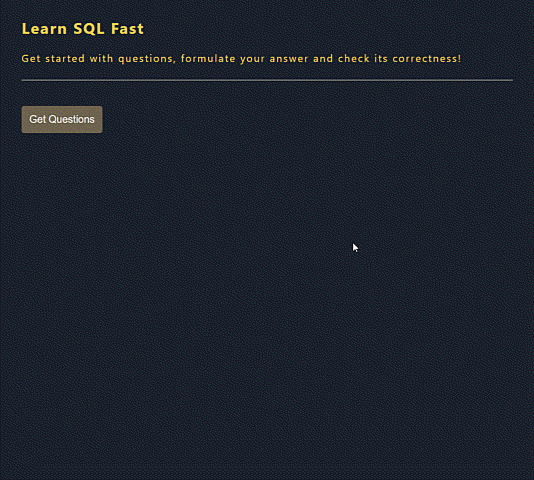
- User click Get Questions button what pulls questions down to the application.
- Each question and answer is hidden. We can click on the proper links to unhide question.
- User can unhide question first, formulate its answer, then unhide the app's answer in order to comapre.
Features:
- NodeJS - server-side API sevice to handle application's HTTP requests.
- MongoDB Atlas - server connects cloud data storage where I keep question-answer documents that are pulled to application.
- RactJS - front-end.
- ExpressJS - web framework that supports building API interfaces.
Setup
No specific installation required.
- npm
- ReactJs
- ExpressJS